Anomaly Detection

Ever since the online transaction is made possible there are millions of credit card fraud victims and every year these frauds are increasing exponentially.

There are many reasons for such fraudulent transaction

1. Lost or stolen
2. Card not received
3. Counterfeited card
4. Remote purchase
5. Card ID Theft

Objective- In this project we are going to take the credit card fraud detection as the case study for understanding this concept in detail.

Introduction-

Anomaly detection is a technique used to identify unusual patterns that do not conform to expected behavior, called outliers. It has many applications in business, from intrusion detection (identifying strange patterns in network traffic that could signal a hack) to system health monitoring (spotting a malignant tumor in an MRI scan), and from fraud detection in credit card transactions to fault detection in operating environments.

Why Classification? Classification is the process of predicting discrete variables (binary, Yes/no, etc.). Given the case, it will be more optimistic to deploy a classification model rather than any others.

Steps Involved

1. Importing the required packages into our python environment.
2. Importing the data
3. Processing the data to our needs and Exploratory Data Analysis
4. Feature Selection and Data Split
5. Building six types of classification models
6. Evaluating the created classification models using the evaluation metrics

Importing Dataset

Pre-Processing:

Observations- The data set is highly skewed, there are 1,142 frauds out of 10,48,575 transactions, I’m considering a sample of 0.1 for our analysis without losing outlier fraction for further unsupervised learning. The outlier fraction is 0.001090.This resulted in only 0.109% fraud cases. This skewed set is justified by the low number of fraudulent transactions.

## Take some sample of the data

df1= df.sample(frac = 0.1,random_state=1)

df1.shape

Exploratory Data Analysis

Finding the out shape of total fraud and valid/ normal transaction.

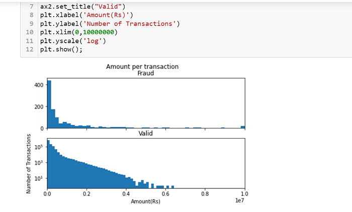
Classification of kind of transaction

Based on above transaction classification, graph presents of amount per transaction.

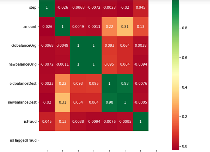
What is a Correlation Matrix?

A correlation matrix is simply a table which displays the correlation coefficients for different variables. The matrix depicts the correlation between all the possible pairs of values in a table. It is a powerful tool to summarize a large dataset and to identify and visualize patterns in the given data.

A correlation matrix consists of rows and columns that show the variables. Each cell in a table contains the correlation coefficient.

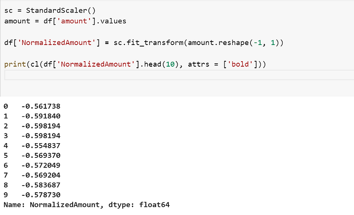
While seeing the statistics, it is seen that the values in the ‘Amount’ variable are varying enormously when compared to the rest of the variables. To reduce its wide range of values, we can normalize it using the ‘StandardScaler’ method in python.

Feature Selection & Data Split

In this process, we are going to define the independent (X) and the dependent variables (Y). Using the defined variables, we will split the data into a training set and testing set which is further used for modeling and evaluating. We can split the data easily using the ‘train_test_split’ algorithm in python.

Modeling

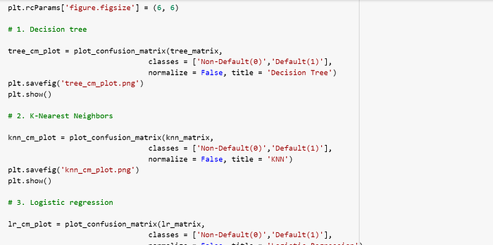
In this step, we will be building five different types of classification models namely Decision Tree, K-Nearest Neighbors (KNN), Logistic Regression, Random Forest, and XGBoost. Even though there are many more models which we can use, these are the most popular models used for solving classification problems. All these models can be built feasibly using the algorithms provided by the scikit-learn package. Only for the XGBoost model, we are going to use the xgboost package. Let’s implement these models in python and keep it in mind that the algorithms used might take time to get implemented.

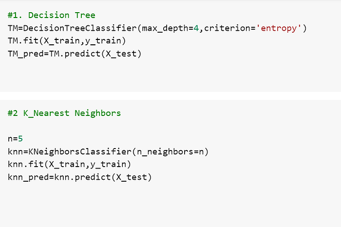
Starting with the decision tree, we have used the ‘DecisionTreeClassifier’ algorithm to build the model. Inside the algorithm, we have mentioned the ‘max_depth’ to be ‘4’ which means we are allowing the tree to split four times and the ‘criterion’ to be ‘entropy’ which is most similar to the ‘max_depth’ but determines when to stop splitting the tree. Finally, we have fitted and stored the predicted values into the ‘tree_pred’ variable.

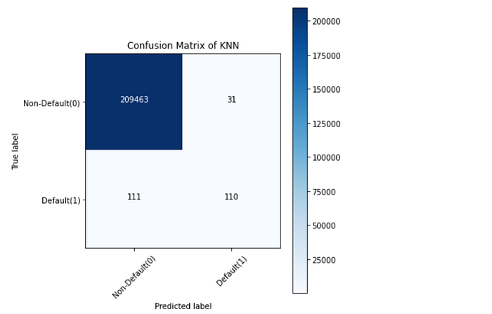
Next is the K-Nearest Neighbors (KNN). We have built the model using the ‘KNeighborsClassifier’ algorithm and mentioned the ‘n_neighbors’ to be ‘5’. The value of the ‘n_neighbors’ is randomly selected but can be chosen optimistically through iterating a range of values, followed by fitting and storing the predicted values into the ‘knn_pred’ variable.

There is nothing much to explain about the code for Logistic regression as we kept the model in a way more simplistic manner by using the ‘LogisticRegression’ algorithm and as usual, fitted and stored the predicted variables in the ‘lr_pred’ variable.

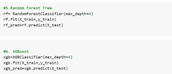
The next model is the Random forest model which we built using the ‘RandomForestClassifier’ algorithm and we mentioned the ‘max_depth’ to be 4 just like how we did to build the decision tree model. Finally, fitting and storing the values into the ‘rf_pred’. Remember that the main difference between the decision tree and the random forest is that, decision tree uses the entire dataset to construct a single model whereas, the random forest uses randomly selected features to construct multiple models. That’s the reason why the random forest model is used versus a decision tree.

Our final model is the XGBoost model. We built the model using the ‘XGBClassifier’ algorithm provided by the xgboost package. We mentioned the ‘max_depth’ to be 4 and finally, fitted and stored the predicted values into the ‘xgb_pred’.

With that, we have successfully built our five types of classification models and interpreted the code for easy understanding. Our next step is to evaluate each of the models and find which is the most suitable one for our case.

Evaluation

In this process we are going to evaluate our built models using the evaluation metrics provided by the scikit-learn package. Our main objective in this process is to find the best model for our given case. The evaluation metrics we are going to use are the accuracy score metric, f1 score metric, and finally the confusion matrix.

1. Accuracy score

Accuracy score is one of the most basic evaluation metrics which is widely used to evaluate classification models. The accuracy score is calculated simply by dividing the number of correct predictions made by the model by the total number of predictions made by the model (can be multiplied by 100 to transform the result into a percentage). It can generally be expressed as:

Accuracy score = No.of correct predictions / Total no.of predictions

Let’s check the accuracy score of the five different classification models we built. To do it in python, we can use the ‘accuracy_score’ method provided by the scikit-learn package.

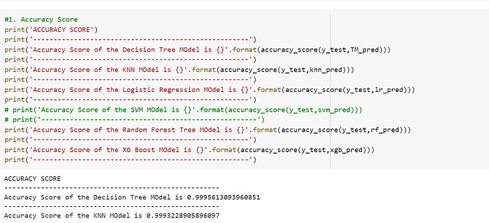
According to the accuracy score evaluation metric, the XG BOOST model reveals to be the most accurate model and the Logistic regression model to be the least accurate model. However, when we round up the results of each model, it shows 0.99 (99% accurate) which is a very good score.

2. F1 Score

The F1 score or F-score is one of the most popular evaluation metrics used for evaluating classification models. It can be simply defined as the harmonic mean of the model’s precision and recall. It is calculated by dividing the product of the model’s precision and recall by the value obtained on adding the model’s precision and recall and finally multiplying the result with 2. It can be expressed as:

F1 score = 2( (precision * recall) / (precision + recall) )

The F1 score can be calculated easily in python using the ‘f1_score’ method provided by the scikit-learn package.

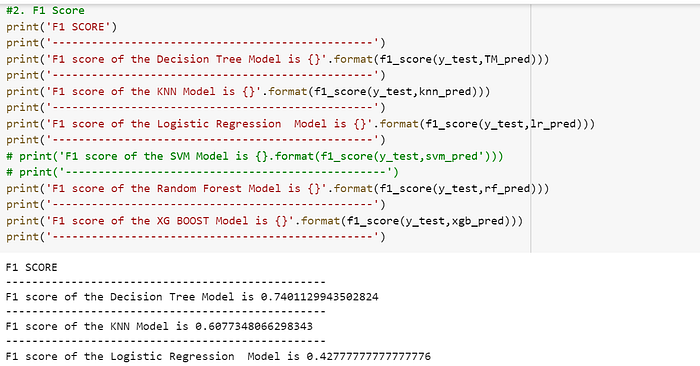
The ranking of the models is almost similar to the previous evaluation metric. On basis of the F1 score evaluation metric, the XG BOOST model snatches the first place again and the Random Forest model is the least accurate model.

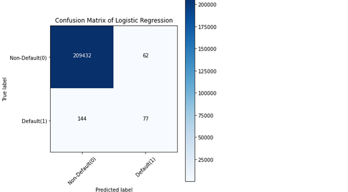
3. Confusion Matrix

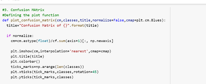
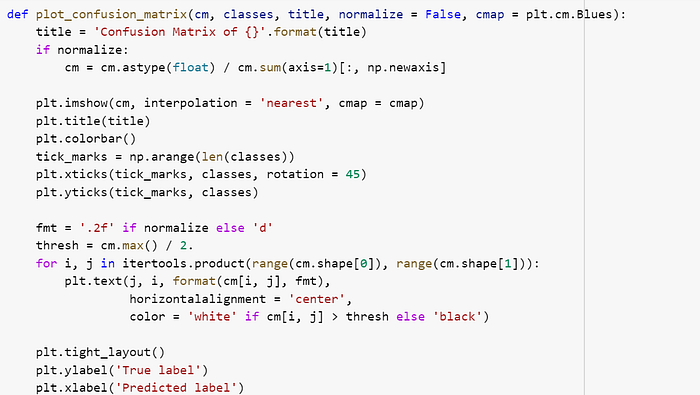
Typically, a confusion matrix is a visualization of a classification model that shows how well the model has predicted the outcomes when compared to the original ones. Usually, the predicted outcomes are stored in a variable that is then converted into a correlation table. Using the correlation table, the confusion matrix is plotted in the form of a heatmap. Even though there are several built-in methods to visualize a confusion matrix, we are going to define and visualize it from scratch for better understanding.

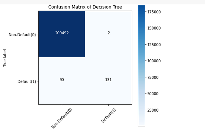
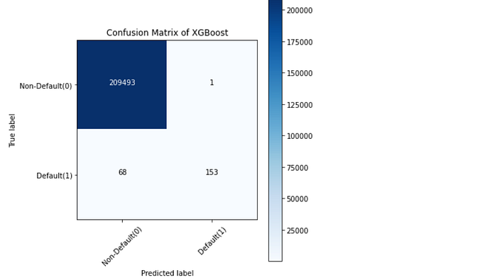
Understanding the confusion matrix: Let’s take the confusion matrix of the XGBoost model as an example. Look at the first row. The first row is for transactions whose actual fraud value in the test set is 0. As you can calculate, the fraud value of 209493 of them is 0. And out of these 209494 non-fraud transactions, the classifier correctly predicted 209496 of them as 0 and 1 of them as 1. It means, for 209493 non-fraud transactions, the actual churn value was 0in the test set, and the classifier also correctly predicted those as 0. We can say that our model has classified the non-fraud transactions pretty well.

Let’s look at the second row. It looks like there were 221 transactions whose fraud value was 1. The classifier correctly predicted 68 of them as 1, and 153 of them wrongly as 0. The wrongly predicted values can be considered as the error of the model.

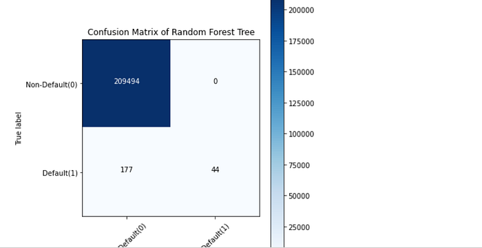
Like this, while comparing the confusion matrix of all the models, it can be seen that the XG Boost Neighbors model has performed a very good job of classifying the fraud transactions from the non-fraud transactions followed by the XGBoost model.

Final Thoughts!

After a whole bunch of processes, we have successfully built five different types of classification models starting from the Decision tree model to the XGBoost model. After that, we have evaluated each of the models using the evaluation metrics and chose which model is most suitable for the given case.

For full code — https://github.com/lolithasherley7/Anomaly-Detection